This is a short introduction to Spectral volume reconstruction and involved partitioning of simplex. We explain what is Spectral volume reconstruction, why the partition is so important, and what is the criteria for judging the partitions. In the end, we give a few partitions (which are best so far) for the one, two, and three-dimensional simplex.
Spectral volume reconstruction is a procedure to construct an approximate function (mostly polynomials) based on averages of target function u(x,y,z) over certain volumes. Given a mesh, the traditional finite volume reconstruction uses averages on neighboring cells to recover the approximation function, while Spectral volume reconstruction uses averages of certain sub-cells of each cell. There are basically two steps for Spectral volume reconstruction on simplex:
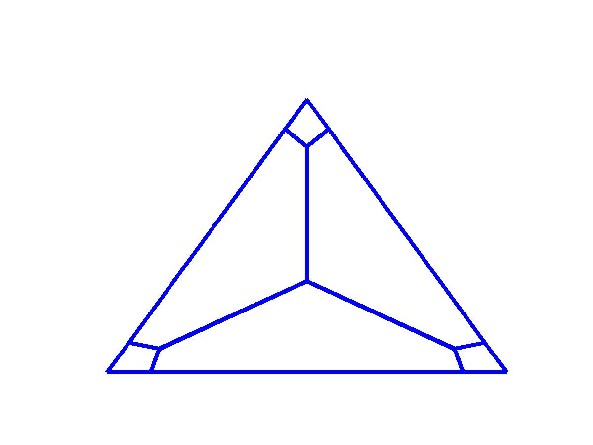
The Lebesgue constant is usually used to measure the error of spectral volume reconstruction. Every simplex can be mapped to a standard simplex, and the Lebesgue constant is invariant under the linear transformation. A sample second-order partition of triangle is shown in the figure below.
Another issue of the spectral volume reconstruction is the computational cost when being used in the spectral volume method. Since flux needs to be computed on each face of the sub-cells, the cost is roughly proportional to the number of faces (edges in 2D) of the partition. So partitons with small Lebesgue constant and small number of faces are desirable.
Unlike polynomial interpolation, for which one only needs to pick the interpolation points after the approximation space is fixed, we have too much freedom in building partitions for simplex. For example, one could even use the union of a few disjoint pieces as one sub-cell. It is really not trivial to come up with a systematic partitioning strategy.
Our idea is inspired by Voronoi diagram. We first pick up certain interpolation points on the simplex, then build a Voronoi diagram for these points. The Voronoi diagram is actually a partition of the simplex. Then the partition optimization becomes a game of moving around the interpolation points.
In 2D Voronoi diagram, the circumcenters of Delauney triangulation are used as the Voronoi vertices. In order to improve the accuracy of spectral volume reconstruction, we can use other points inside those triangles too. Numerical experiments did show some decrease in the Lebesgue constants. Similar ideas also work for three dimensional simplex.
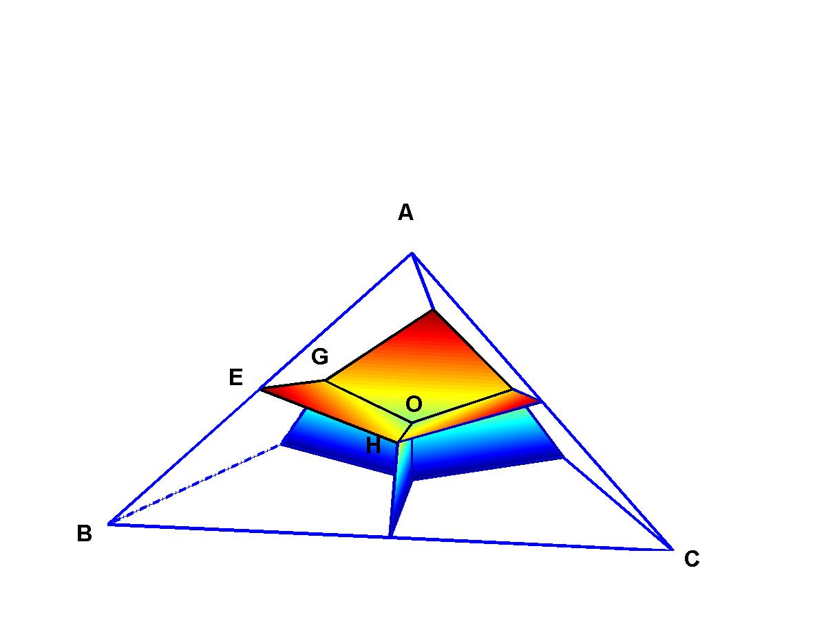
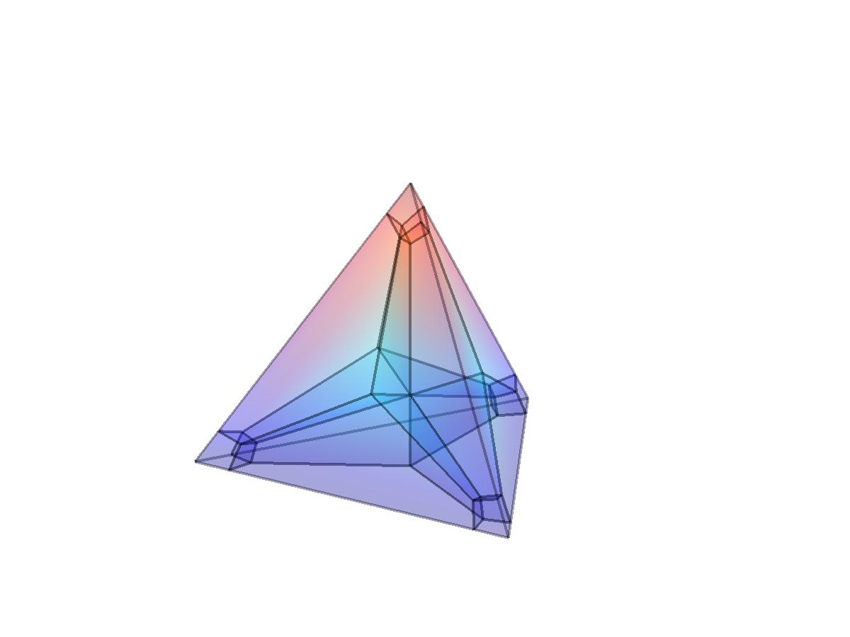
An optimzed first-order and second-order partition of tetrahedron is shown in the following figure.
Some 2D and 3D optimzied partition data can be downloaded in the following. The data files are pretty well self-explained. See [1] for information on optimized 1D partitions.
Note: all the partition vertices are given in its bary-center coordinates if not specified otherwise.
2D partitions: