S501 HW8 SOLUTIONS

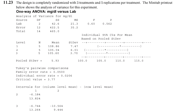
c Homoscedasticity means equal variances in the three labs, or, in more practical terms, equal variability or scatter in the measurements from the labs. In this case H₀ was not rejected, so the three labs are all giving the same (population) mean. Thus, if each lab would make many replicate measurements, the average of those measurements would be the true m . Severe heteroscedasticity would mean that at least one lab would have a much higher variance than one or both of the others. Thus, even though replicate measurements from that lab would average out to the correct m , they would be much more scattered about the mean than replicate measurements from the other lab(s). In other words, the measurements from the lab with higher variance are not as reliable as those from labs with lower variance. To put it somewhat differently, the higher the variance, the worse the precision.

d If each patient contributed a sample to all three labs, then we would have a randomized block design (RBD) with the patients as blocks and labs as treatments. Suppose the patients’ samples were given to the labs as indicated below. Since this is a RBD it must be analyzed as such rather than as a one-way ANOVA. The analysis is given below.

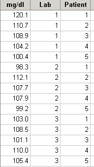
The F-test for treatment effects (F = .56, P = .590) shows that H₀(treatments) should not be rejected, thus there is no evidence of effects due to labs; similarly the F-test for blocks (P = .5596) shows that there are no block effects.

DIAGNOSTICS

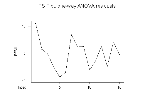
TS PLOTS: The time series plot for the one-way ANOVA (below) shows a slightly suspicious "wave" pattern, but this is likely due to the small number of residuals – the eye tends to make patterns out of a small number of points. So, in itself, this plot seems consistent with independence of the observations. Also, it is consistent with homoscedasticity: there is no funneling, bulging, squeezing, etc.

The same is true for the TS plot of the RBD residuals (not shown here): the plot looks almost the same as for the one-way ANOVA.

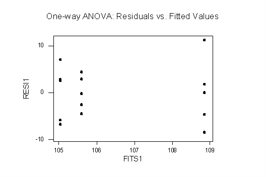
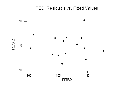
Plots of Residuals vs. Fitted Values: both plots are consistent with homoscedasticity: in the one-way plot there is only a slight difference in vertical spreads and one point that looks like an outlier (but a boxplot shows that it is not an outlier). The RBD plot shows no evidence of funneling, etc.

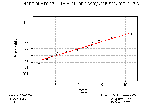
NORMAL PROBABILITY PLOTS: the plot for the residuals from the one-way ANOVA (below) is consistent with the assumption of normality. The points hug the straight line closely, and the Anderson-Darling P-value of .777 indicates that the hypothesis of normality should not be rejected, which is consistent with the visual impression. The normal prob. plot for the RBD residuals (not shown) is also consistent with normality: the points also hug the straight line and Anderson-Darling P = .760.

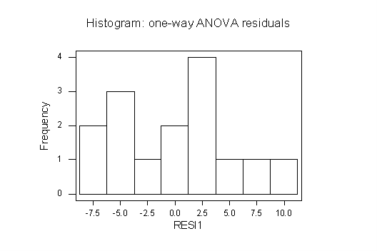
HISTOGRAMS: the histogram for the one-way residuals (below) looks at best only vaguely like a bell-shaped normal curve, but this is most likely due to the small number of residuals. The histogram of the RBD residuals (not shown) looks even worse, and for the same reason. Because of the small number of residuals, these histograms cannot be expected to be very informative.

Summary of diagnostics: Because of the small number of residuals, neither the histograms nor the TS plots are very informative. The plots of residuals vs. fitted values are consistent with homoscedasticity; likewise the normal probability plots are consistent with normality. Thus we can be confident that the results of the analyses are reliable. But: it is important to use the correct analysis. If the experiment was run in randomized blocks, that is the analysis that must be used.

Limitations: Original problem: (1) If the samples all come from one person, the performance of the labs on different people cannot be assessed. (2) It is not clear what the values should be for a person who has drunk 50 mg glucose. The labs are consistent with each other -- that's what the analysis tells us -- but are they all equally accurate or equally inaccurate? (3) We don't know from the problem how the samples were assigned to the labs. Was it in random order, etc.? For instance, it would be a bad design if the first 5 samples went to lab 1, the second 4 to lab 2, etc. The order should be randomized. (4) We have no idea of the probability of making a type II error in this situation. (We have not dealt with such questions in this course, but it is an issue that has to be addressed.)

Conclusion: In either scenario the analysis indicates that the three labs are giving consistent results. They are all estimating the same quantity and there is no evidence of differences in variability (i.e., precision) between the labs. hence a decision between the labs would have to be based on some other criterion than accuracy or precision, e.g., cost, service, timeliness, etc.