Now X is just R^3. In this case, there's a cheap way to get your hands on C. It's easiest to describe when U is actually the subgroup of totally positive units, and instead of X we take the "totally positive octant," the subset Y of X consisting of the points with all embeddings positive. Then one can take all the units in Y and can take their convex hull. This gives an unbounded polyhedron P with facets that are finite polygons, and one can decompose the space Y into rational cones by taking the cones on the facets of P. By taking a subset of the cones of this decomposition, one gets the desired set C.
The following pictures illustrate this for the real cubic field of discriminant 49. This field is actually the totally real subfield of the cyclotomic field Q(zeta_7), and it's the first field in lists ordered by discriminant. Given this information it's easy to compute that the generating polynomial is x^3-x^2-2*x+1. If t is a root of this polynomial, then the two generators of the totally positive units are u=t^2 and v=(t+1)^2. So we need to compute the convex hull of all points of the form u^a v^b, where a,b are integers.
To do this and to generate some pictures, we use gp, qhull, and geomview. The program gp needs no introduction, and it's clearly perfect for doing arithmetic in a number field. To get the floating point representation in Minikowski space, the obscure element .nf[5][1] of a bnf is useful (surely this element needs a member name of its own). After producing a list of points, we feed it into qhull, a convex hull computing program. We use qhull (instead of porta) because it deals with floating point vertices, and because it can generate output that geomview understands (if you invoke it with "qhull -G"). Finally the geomview program can take the qhull output and display it interactively. This means one can zoom in on polyhedra, rotate them, fly around them, all kinds of stuff. Finally we can save the pictures from geomview, and can then use a program like xv or gimp to clean them up.
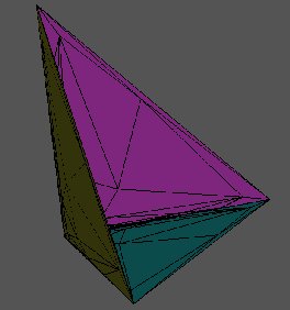
Figure 1 shows a portion of P, as viewed from the origin. The apparent symmyetry is induced from permuting the real places of F. The point in the center of the figure is the unit 1. The three vertices of the figure correspond to the three coordinate axes in X, and you can see that the triangles are flattening out to the coordinate planes as they get further away from 1.
The units u and v are two of the vertices of one of the triangles containing 1; in fact, they're the other two vertices of the purple triangle that borders a blue triangle (so it's due west of 1). The other purple triangle that contains the edge (u,v) has as its third vertex uv. For the fundamental domain C, one can take the union of the two cones (1,u,v) and (u, v, uv), and can then delete certain cones where the edges and vertices are glued together by the unit action.
Figure 1: A small piece of P seen from the origin |
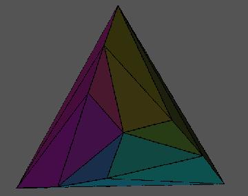
Figure 2 shows more of P. Note how the triangles become long and thin as they approach the coordinate axes. Also the flattening of the triangles near the coordinate planes is more pronounced, and one clearly sees how the polyhedron asymptotically looks like the octant Y.
Figure 2: More of P |
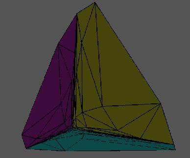
Figure 3 shows even more of P. This time we move away from the origin and swing around behind P.
Figure 3: Even more of P |